Shaded Ride

Project:

Date:

Team:

Keywords:

Mapping the Shading Level of Bike Lanes in Amsterdam with Deep Learning and Google Street View Images

2023.11

Biru Cao, Maoran Sun

Thermal Comfort, Street View Image, Shade Provision, Deep Learning

Trees and buildings can generate shade and increase thermal comfort in hot weather, which is essential for cyclists. This research chose Amsterdam as the study area as one of the world’s most bicycle-friendly cities with over 500 km of bike lanes. The study investigates how the trees and buildings contribute to the shade provision of bike lanes and calculates their level of shadiness. A ‘Shade Index’ is employed to quantify the level of shadiness on streets, defined as the ratio of the unobstructed sky area to the total sky area. Deep learning techniques are utilized to calculate this index by analyzing selected street view images from specific locations along the bike lanes. The study identifies street trees and building blocks as the primary sources of sky obstruction and shade provision. Consequently, a shade rating map of Amsterdam’s bike lanes is generated, offering cyclists an alternative to the shortest routes typically suggested by map applications, particularly those preferring cooler, shaded routes during hot weather.

Data

Cycle lane

Cycle path

Cycle track

Figure 1: Different types of bike lanes in Amsterdam

For this study, we focused on the city of Amsterdam, the capital of the Netherlands, renowned for its extensive cycling culture and infrastructure. The city’s preference for cycling extends beyond cultural affinity and reflects a collective agreement to prioritize this mode of transportation. Amsterdam boasts approximately 515 km of dedicated cycling infrastructure, encompassing bike lanes, paths, and elevated tracks (Figure. 1.).

# try which_result=1 or =2 to get polygon boundary or only a centeral point
# network_type will simplify the network

cf = '["cycleway"]'

G = ox.graph_from_place('amsterdam, netherlands', custom_filter=cf)

G_projected = ox.project_graph(G)
# defalut, epsg:4326, uncomment to use local projection crs, e.g., epsg:32630

Get bike lanes network

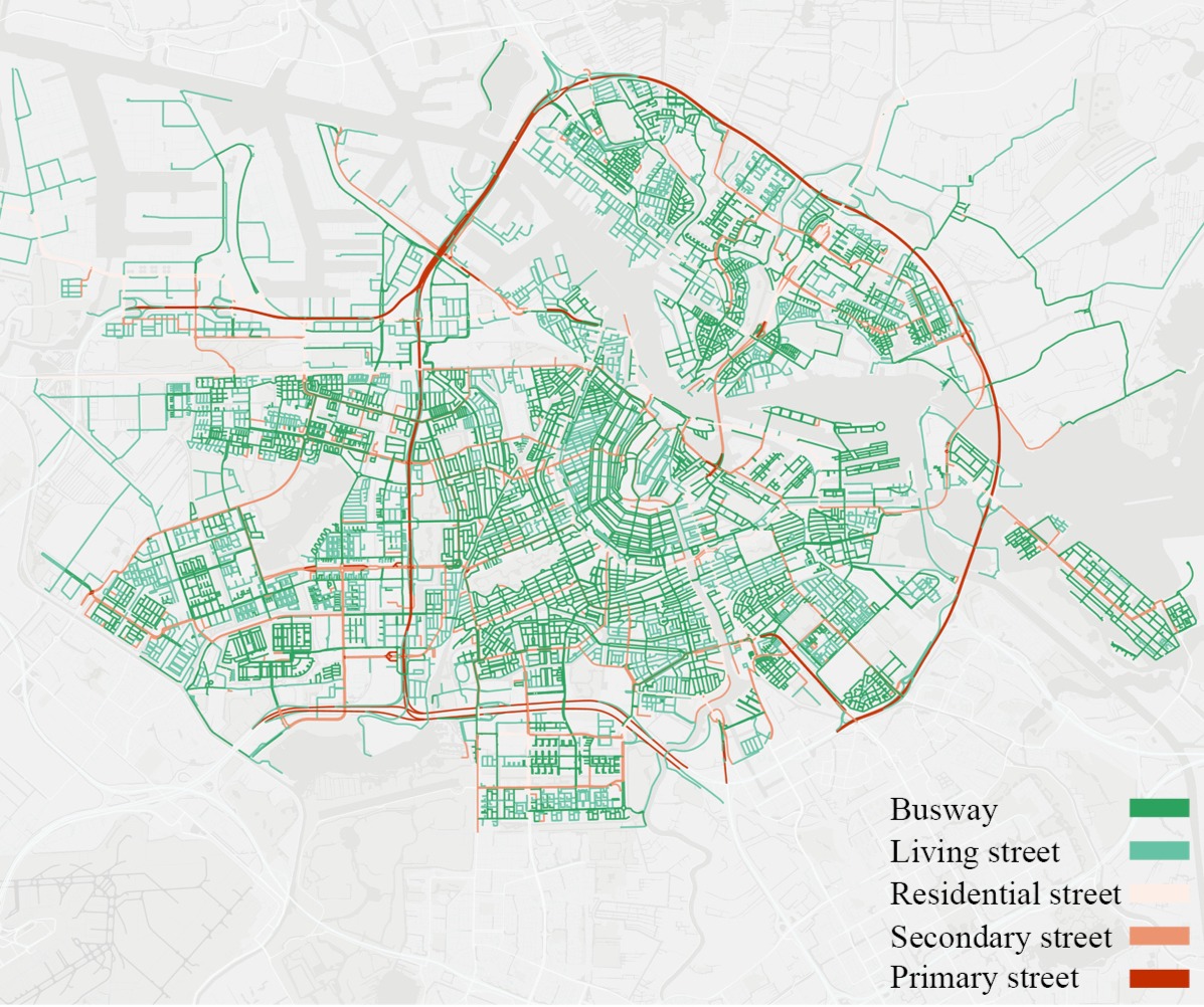
Figure 2: Amsterdam’s road map

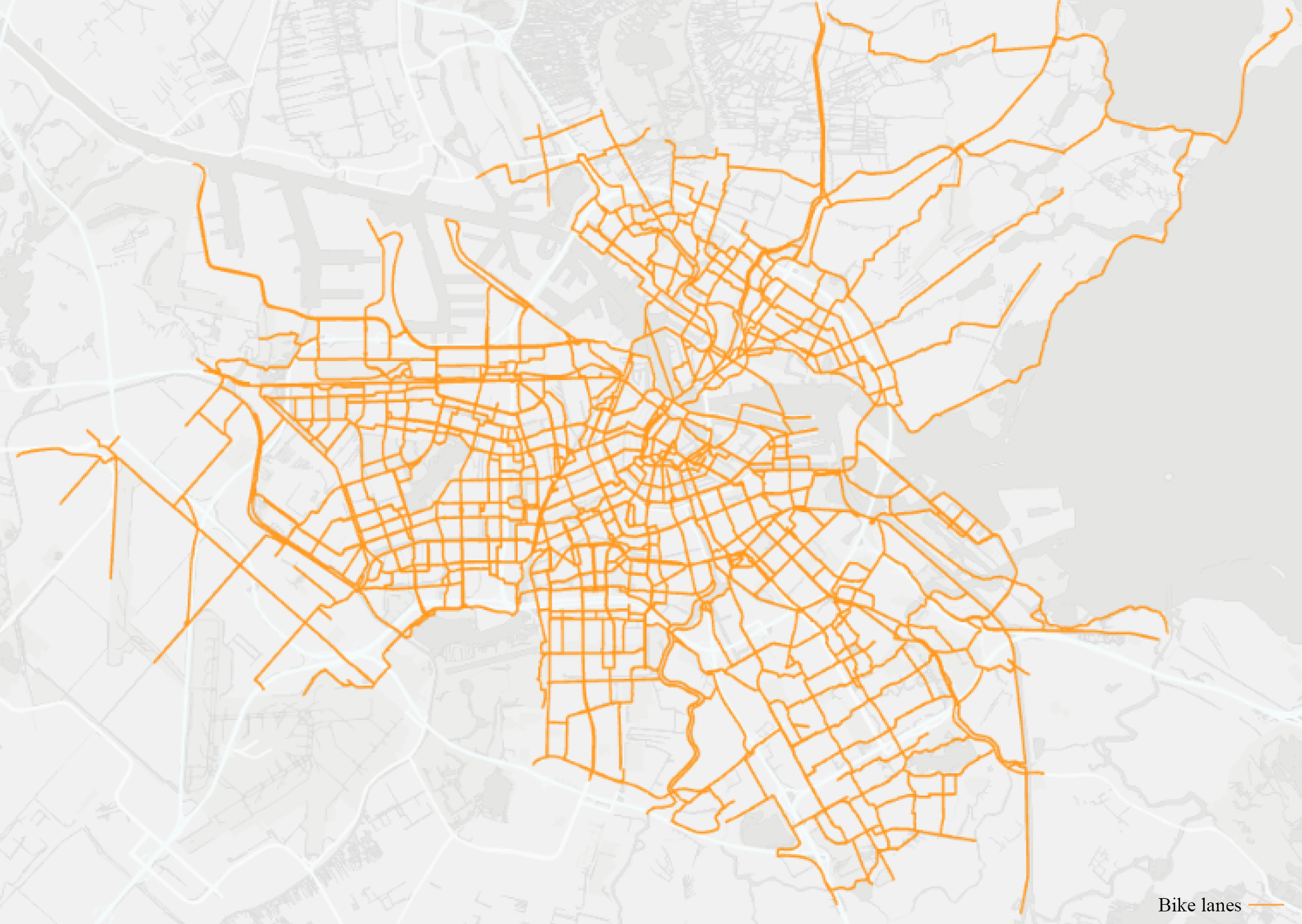
Figure 3: Amsterdam’s bike lane map

The task of classifying HtD houses shares lots of similarities with other building energy-related prediction tasks, such as building energy consumption, efficiency, and ratings. In this subsection, we present reviews of methods
for building-level energy predictions. The main data sources employed in this research encompass street network, bike lane network and street view images

Street network
The road map of Amsterdam was sourced from Open Street Map1 using the OSMnx Python package to download (Figure 2).

Bike lane network
Bike lane data was obtained from the Amsterdam Walking and Cycling Network Dataset available on the City’s open data portal2. This dataset comprises a network of roads for walking and cycling in Amsterdam and its surrounding area. As the original dataset includes routes for both pedestrians and cyclists, bike lanes were further isolated and extracted from the dataset (Figure 3). To achieve a finer-grained cycling network, bike lanes were further segmented at the intersection points between each other.

Street view images
Street view images are widely used in studies examining people’s perceptions of the built environment. GSV images, which cover more than 100 countries, were chosen as an ideal data source for this study setting. GSV images were retrieved from Google Map’s Static Street View API at designated locations and angles. In total, 88,128 GSV images along the bike lanes were collected.

Methods

Figure 4: Street segments and their mid-points

# Get the mid point of every street segment

streets = gpd.read_file("amsStreetSegment.geojson")
streets.head()

def getMidx(g): return np.mean(g.xy[0])
def getMidy(g): return np.mean(g.xy[1])

streets[‘lon’] = streets.geometry.apply(getMidx)
streets[‘lat’] = streets.geometry.apply(getMidy)

streets.to_pickle(“streetPt.p”, protocol=3)

Get request points

Google Street View Image Collection

GSV images can be requested by specifying the image size, location coordinates, field of view, and heading angle through Google Map’s API. Midpoints from each segment were extracted as the sampled location coordinates
for GSV retrieval (Figure 4).

Most deep learning-based semantic segmentation models are trained with perspective images, so GSV images were obtained in perspective view instead of panoramas. Four images pointing north, west, south, and east (heading angle of 0, 90°, 180°, 270°) were downloaded for each location coordinate to represent the environment of that specific point (Figure 5). Other parameters for the GSV API, such as field of view and pitch, were kept at default values, which are 90 for field of view and 0 for pitch. The capture dates of each GSV image were also considered during the download process. As shade is more appreciated by cyclists during the summer season, only GSV images taken in June, July, August, and September were requested. Due to some images being missing at certain times of the year, the time frame of the GSV images.

def GSV_meta_single(lat, lon, apiKey):

# original request url for API call
meta_url = "https://maps.googleapis.com/maps/api/streetview/metadata?size=600x400&location={},{}&key={}"

# format the request url with feeded parameters
request_url = meta_url.format(lat, lon, apiKey)

try:
# request and format the metadata
response = requests.get(request_url).json()
# return metadata if GSV exists
return {'date':response['date'], 'lat':response['location']['lat'], 'lon':response['location']['lng'], 'panoID':response['pano_id']}

Get pano IDs

Figure 5: Examples of GSV image and segmentation of four directions

Shade Index Calculation

The sky view factor (SVF) measures the proportion of the visible sky or open canyon space in urban street canyons (Chapman and Thornes, 2004). While the calculation of SVF typically involves panoramic photography and geometric calculation, this study introduces a similar index to quantify shading effectiveness in a more efficient workflow using deep learning, the “Shade Index”. This index is defined as the ratio of the number of non-obstructed sky pixels to the total number of image pixels in a street view image. Given that trees and buildings are the two main factors contributing to sky obstruction, their combined contribution to shade is calculated. This index, ranging from 0 to 1, represents the ratio between the area of the unobstructed sky and the total sky area, indicating a fully enclosed and open street sky.

More specifically, we applied a scene parsing model pre-trained on the ADE20K dataset (Zhou et al., 2017), a large-scale scene-centric dataset containing images annotated with pixel-level objects and object parts labels in 150 semantic categories, including sky, buildings, trees, sidewalks, and cars.

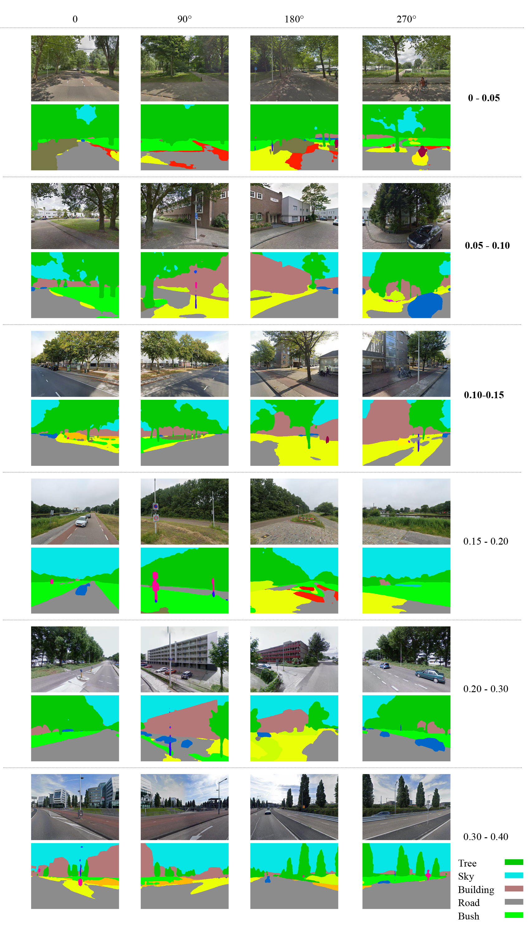
Figure 6: Selected segmented GSV images

Shaded Bike Lane Generation
In this study, the 150 categories were consolidated into four distinct groups for a more simplified and clear result: tree canopy, building block, non-obstructed sky, and others. With the Shade Index calculated for all the selected points, it was possible to determine which bike lanes could be considered shaded and filter them accordingly.

A total of 16,485 locations’ Shade Index values were computed, ranging from 0 to 0.81, with an average value of 0.21. The majority of the values were distributed within the 0-0.5 range. This range was further subdivided into smaller intervals with a gap of 0.1 for more detailed analysis, as these represented the more shaded indexes. A detailed comparison between the Shade Index and the shade present in the GSV images revealed that a site could be considered effectively shaded if the value falls between 0-0.15 (Figure 6). The GSV images showed that shades were created by either tree canopies or building blocks, or a combination of both.

Therefore, points with a Shade Index falling within the 0-0.15 range were selected. The index, along with their geometric information, was joined to the street segments.

Results

Amsterdam’s average Shade Index value is 0.21, with a median of 0.20. When considering the range of 0-0.15, which is defined as “shaded” cycle routes, the mean is 0.09, and the median is 0.10 (Figure 7). The Shade Index map (Figure 8) reveals that the central part of the study area generally has a higher index value than the periphery. This is likely due to the higher building density in the city center, where taller buildings cast larger shadows, thereby contributing to a higher Shade Index. In contrast, areas with less dense and lower buildings might exhibit a lower Shade Index. The distribution of the Shade Index between 0-0.15 appears quite even, suggesting that cyclists have a high likelihood of finding a more shaded route in most parts of Amsterdam.

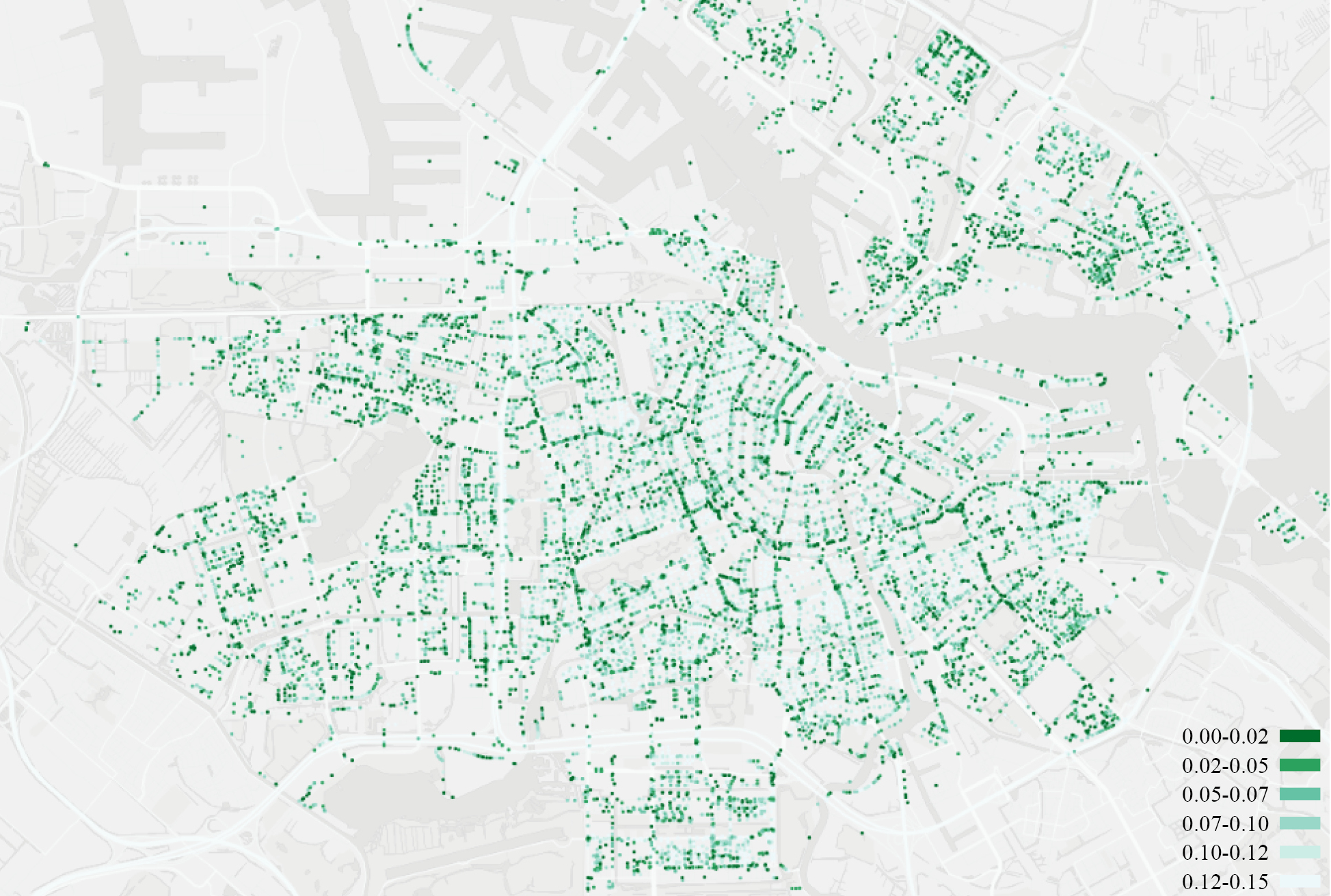
Figure 7: Shade Index map of Amsterdam

Similarly, it can be observed that the central part of the study area has more shaded bike lanes compared to the rest of the study area (Figure 9). The shaded bike lane network in Amsterdam-Noord (North Amsterdam, separated by the IJ, a body of water) is more scattered compared to the southernpart.

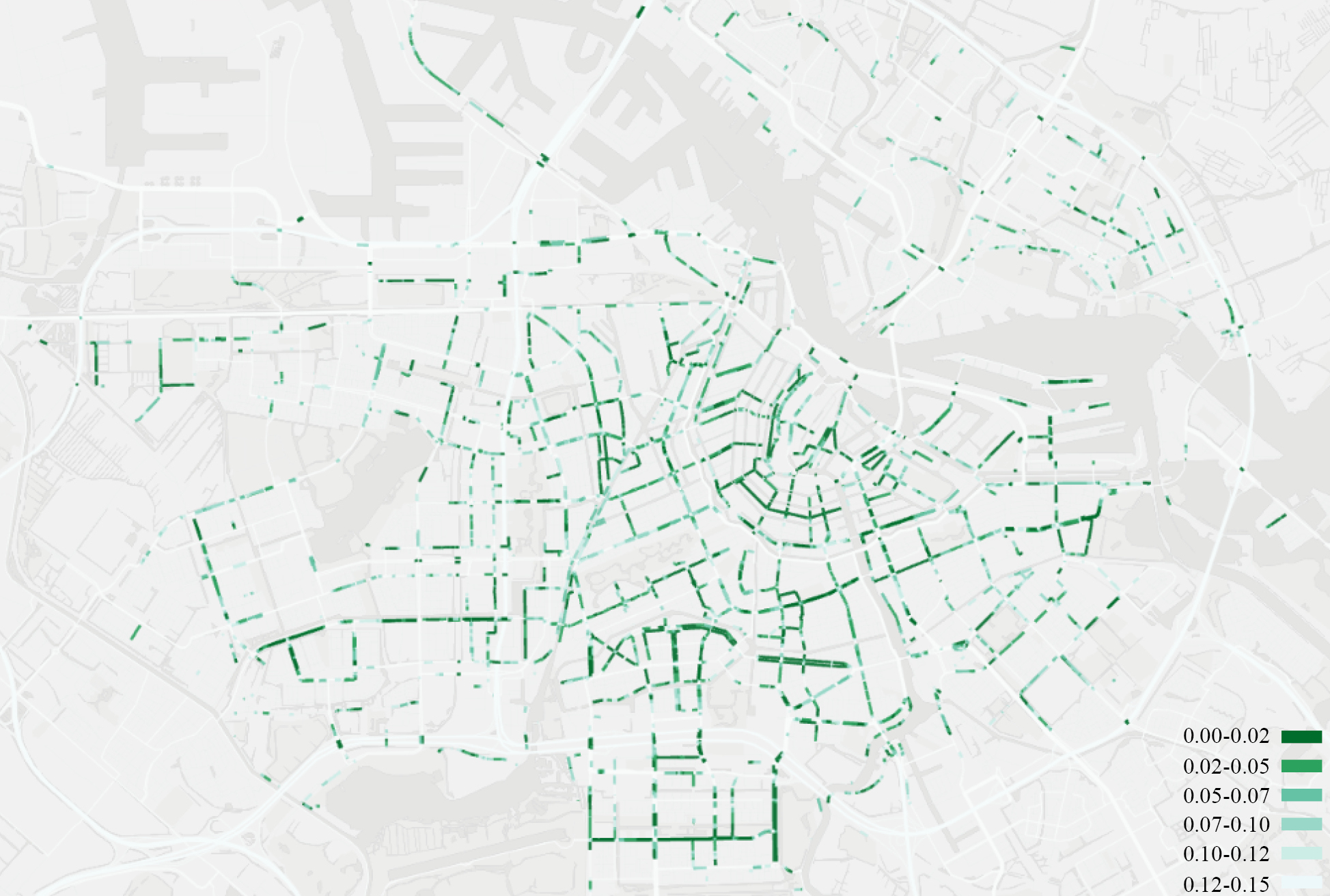
Figure 8: Shaded bike lanes

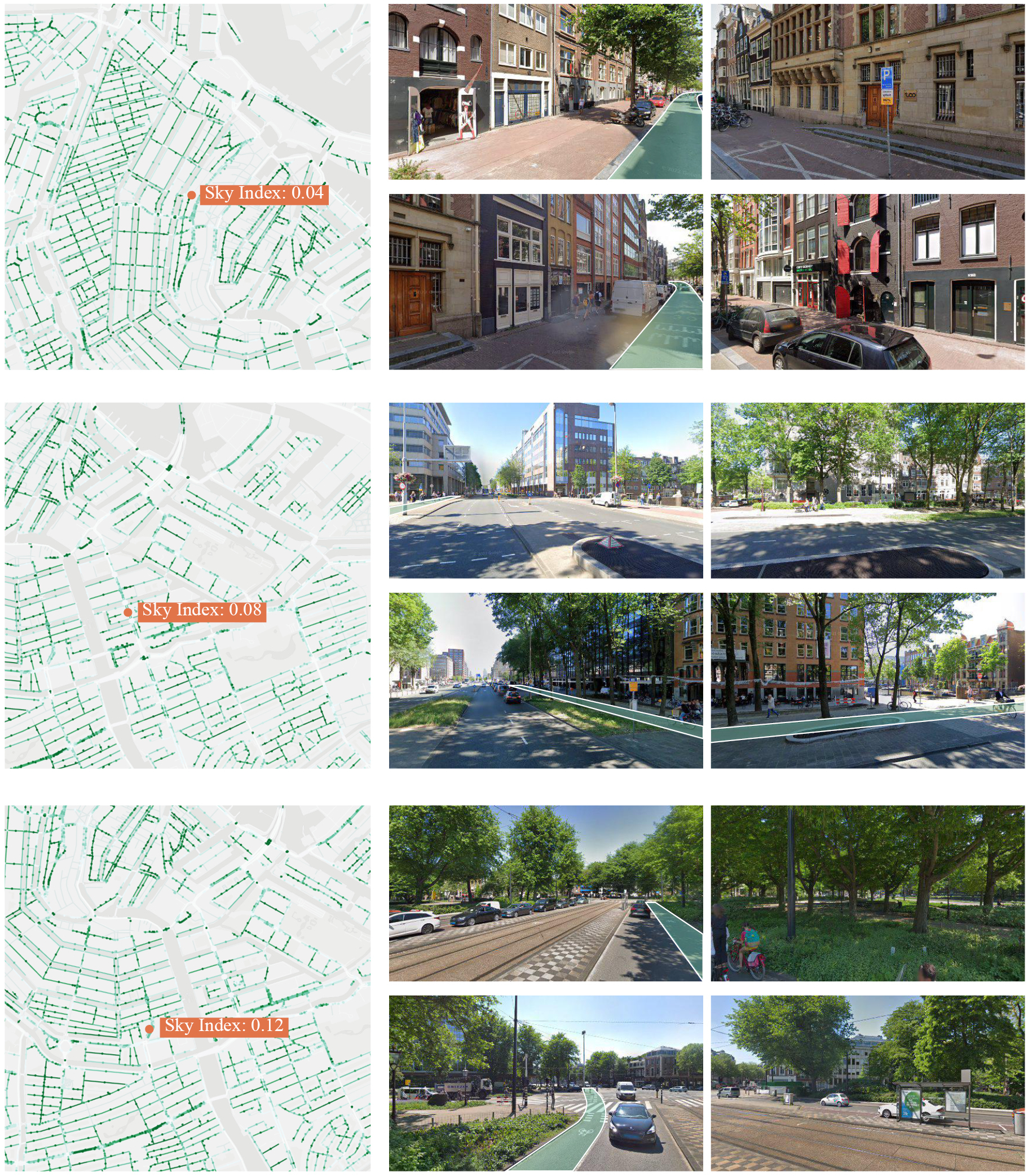
Three random locations were selected to verify whether the calculation of shade effectiveness aligns with the actual physical environment. These 17 spots are distributed along the following bike trails: Spuistraat, Weespeplein, and Frederiksplein, and were examined (Figure 10). Upon reviewing each location’s GSV images, it was found that the results of the Shade Index corresponded well with each spot’s true surrounding environment.

This further substantiates the assertion that if a street’s Shade Index is below 0.15, it can provide sufficient shade to ensure thermal comfort.

Examination

Figure 9: GSV images for examining the Shade Index values, from top to bottom: points
along Spuistraat, Weesperplein, and Frederiksplein bike trails

Conclusion

In conclusion, this research presents a workflow for evaluating the combined shading effects of trees and buildings using street view images. A deep learning-based approach was employed to segment the images and calculate the Shade Index of selected locations. Utilizing 65,942 GSV images, the Shade Indexes for 16,485 bike lane segments were calculated. The final outcome, a map of shaded cycle paths, could assist cyclists in choosing routes with a higher Shade Index to avoid direct sunlight and maintain coolness, particularly during the summer months.

This research method demonstrated an efficient workflow in data collection and image processing by leveraging GSV images and deep learning. The method could be applied to other cities where data can also be easily obtained. The use of deep learning’s image segmentation method also enables the classification and Shade Index calculation on a large scale, and the final result was tested and found to be convincing.

Contents